So I currently have a piece of code that only functions on one of the sheets in my workbook. I want to modify it so it can work on any of the sheets.
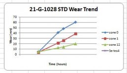
The macro is essentially using relative ranges to graph the data. I have tried solving it myself but can't seem to get it to work, refer to "Error 1". I also run into a second error where when it works on that one sheet, it's graphing an extra "series" I will attach an image of it below- Refer to Error 2
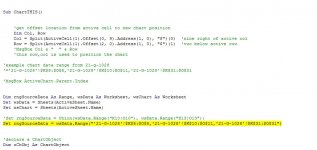
The piece of code I think that needs modifying is:
The second error that I get is, where its graphing an extra "series" I am not sure how to fix that.
The macro is essentially using relative ranges to graph the data. I have tried solving it myself but can't seem to get it to work, refer to "Error 1". I also run into a second error where when it works on that one sheet, it's graphing an extra "series" I will attach an image of it below- Refer to Error 2
Code:
Sub ChartTHIS()


        'get offset location from active cell to new chart position
        Dim Col, Row
        Col = Split(ActiveCell(1).Offset(0, 9).Address(1, 0), "$")(0)  'nine right of active col
        Row = Split(ActiveCell(1).Offset(2, 0).Address(1, 0), "$")(1)  'two below active row
        'MsgBox Col & "  " & Row
        'this row,col is used to position the chart

    'example chart data range from 21-g-1028
    '='21-G-1028'!$K$8:$O$8,'21-G-1028'!$K$10:$O$11,'21-G-1028'!$K$31:$O$31

    'MsgBox ActiveChart.Parent.Index


    Dim rngSourceData As Range, wsData As Worksheet, wsChart As Worksheet
    Set wsData = Sheets(ActiveSheet.Name)
    Set wsChart = Sheets(ActiveSheet.Name)

    'Set rngSourceData = Union(wsData.Range("K10:O10"), wsData.Range("K13:O13"))
    Set rngSourceData = wsData.Range("'21-G-1028'!$K$8:$O$8,'21-G-1028'!$K$10:$O$11,'21-G-1028'!$K$31:$O$31")


    'declare a ChartObject
    Dim oChObj As ChartObject

    'the Add method (of the ChartObjects object) is used to create a new empty embedded
    'chart and add it to the collection (ChartObjects object) in the specified sheet
    Set oChObj = wsChart.ChartObjects.Add(Left:=2, Width:=350, Top:=5, Height:=200)

    'using the Chart Property of the ChartObject object returns a Chart object
    'which refers to a chart
    With oChObj.Chart
    'use ChartType Property of the Chart object to set type of chart - Line with Markers
    .ChartType = xlLineMarkers
    'use SetSourceData Method of the Chart object to set the range of source data for the chart
    .SetSourceData Source:=rngSourceData, PlotBy:=xlRows

    'the Parent property of the Chart object returns its Parent object ie. ChartObject object (oChObj)
    'the ChartTitle object exists and can be used only if the HasTitle property (of the Chart object) is True
    .HasTitle = True
    'get sheet name into chart title:
    .ChartTitle.Characters.Text = ActiveSheet.Name & " STD Wear Trend"

       'calc position of chart relative to active cell
       Col = Split(ActiveCell(1).Offset(0, 9).Address(1, 0), "$")(0)  'nine right of active col
       Row = Split(ActiveCell(1).Offset(2, 0).Address(1, 0), "$")(1)  'two below active row

       'here use the calculated row and col offset to position the chart:
       With .Parent
       'set the embedded chart to be free-floating so that it does not move or size with its underlying cells
       .Placement = xlFreeFloating
       'align the left edge of the embedded chart with the left edge of the worksheet's column B
       .Left = wsChart.Columns(Col).Left
       .Top = wsChart.Rows(VBA.Val(Row)).Top
       'set rounded corners for the embedded chart
       .RoundedCorners = True
       'using the Name Property of the ChartObject object - set the name of the embedded chart to "AnnualSalesProfit"

       End With

        .Axes(xlCategory, xlPrimary).HasTitle = True
        .Axes(xlCategory, xlPrimary).AxisTitle.Characters.Text = "Time (hours)"
        .Axes(xlCategory, xlPrimary).CategoryType = xlTimeScale
        '.Axes(xlCategory, xlPrimary).MinimumScaleIsAuto = True
        '.Axes(xlCategory, xlPrimary).MaximumScaleIsAuto = True

        .Axes(xlValue, xlPrimary).HasTitle = True
        .Axes(xlValue, xlPrimary).AxisTitle.Characters.Text = "Wear (mm)"

            .Axes(xlValue).MinimumScale = 0
            .Axes(xlCategory).MinimumScale = 0
            .Axes(xlCategory).MaximumScale = 4000
            .Axes(xlCategory).MajorUnit = 1000
            .Axes(xlCategory).MinorUnit = 1000
            .Axes(xlCategory, xlPrimary).TickLabels.NumberFormat = "0"

        .SeriesCollection.NewSeries

         Dim col2, row2


         'data series 1 ----- HOW TO CODE RELATIVE DATA RANGES INTO THE CHART MACRO
         'example  active K8   to   Q8
         Col = Split(ActiveCell(1).Offset(0, 0).Address(1, 0), "$")(0)  'nine right of active col
         'this row will always be used as the x axis labels
         Row = Split(ActiveCell(1).Offset(0, 0).Address(1, 0), "$")(1)  'two below active row
         'and K10 to Q10
         col2 = Split(ActiveCell(1).Offset(0, 6).Address(1, 0), "$")(0)  'nine right of active col

        .SeriesCollection(1).XValues = Range("$" & Col & "$" & Row & ":$" & col2 & "$" & Row)
        row2 = Split(ActiveCell(1).Offset(2, 0).Address(1, 0), "$")(1)  'two below active row
        .SeriesCollection(1).Values = Range("$" & Col & "$" & row2 & ":$" & col2 & "$" & row2)
        .SeriesCollection(1).Name = "zone 0"


        'data series 2 -----
        'only the row changes relatively
        row2 = Split(ActiveCell(1).Offset(3, 0).Address(1, 0), "$")(1)  'two below active row
        .SeriesCollection(2).XValues = Range("$" & Col & "$" & Row & ":$" & col2 & "$" & Row)
        'next row down:
        .SeriesCollection(2).Values = Range("$" & Col & "$" & row2 & ":$" & col2 & "$" & row2)
        .SeriesCollection(2).Name = "zone 1"


         'data series 3 -----
        'so you only need to change the row offset and then the other lines are the same:
        'see this one has a long offset of 23
         row2 = Split(ActiveCell(1).Offset(23, 0).Address(1, 0), "$")(1)  'two below active row

        .SeriesCollection(3).XValues = Range("$" & Col & "$" & Row & ":$" & col2 & "$" & Row)
        .SeriesCollection(3).Values = Range("$" & Col & "$" & row2 & ":$" & col2 & "$" & row2)
        .SeriesCollection(3).Name = "zone 12"


      'and you can add as many zones of data as you want...


    'using constant values in MsoChartElementType Enumeration to specify if the chart elements are to be displayed and how to display them
    'Display chart title above chart
    .SetElement msoElementChartTitleAboveChart
    'Display major gridlines along primary value axis
    .SetElement msoElementPrimaryValueGridLinesMajor
    'turn off legend
    '.SetElement msoElementLegendRight

    End With

    End Sub
The piece of code I think that needs modifying is:

Code:
'Set rngSourceData = Union(wsData.Range("K10:O10"), wsData.Range("K13:O13"))
    Set rngSourceData = wsData.Range("'21-G-1028'!$K$8:$O$8,'21-G-1028'!$K$10:$O$11,'21-G-1028'!$K$31:$O$31")
The second error that I get is, where its graphing an extra "series" I am not sure how to fix that.


