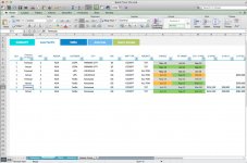
Excel Sheet Setup (Advance)

Jeff,

The revised version works perfectly. Where can I view the hard coded formula/commands you've put in place?

Thanks for all your support.

Han
Also, see if the issue is still happening on the attached file. View attachment 1553.

Apparently some weird stuff can happen to formulas where the column headers contain dates. So I put a 'helper' column in above the column headers, to see if it makes any difference.

EDIT: I just changed my date settings to US format, and this approach seems to work fine.

The issue is that for some obscure reason, if you enter say 1/1/2013 into a table column header, Excel stores it as a string, not a date. If you then tell excel "Apply the date format of MMM-YY to this", then Excel displays 'Jan-13' (which is what we want) but when it converts the string to a date using any of the date-related functions, Excel thinks that this number for some reason relates to the 13th of January 2013.

Way around it is just to have some helper cells one row above. Because they are not table column headers, they are stored as dates, not strings.

Note that you don't need these helper cells in the summary tab, because that summary table doesn't contain any formulas. Also note that no-one will see this extra helper row, because the month-by-month breakdown is only required to be visible in the summary sheet...i.e. you should hide columns T onwards in the data input sheets, like in this version. View attachment 1554
 
When you say "Where can I view the hard coded formula/commands you've put in place? ", do you mean the VBA code (aka Macros) that amalgamate the seperate tables into the summary?

If so, push Alt F11, which will open the Visual Basic Editor, then double click on the Sheet5 (Summary) icon that appears in the left hand side. But if you're not familiar with the VBE, then it will be confusing as hell.

Here's the actual code that does the amalgamating. (Note that the code in Module1 or Module2 doesn't do anything...this was just where I was experimenting. I'll remove those modules and post an updated version soon)
Code:
Private Sub Worksheet_Activate()

    Dim lo As ListObject
    Dim lr As ListRow
    Dim rngSource As Range
    Dim rngDest As Range
    Dim pt As PivotTable
    
    With Application
        .ScreenUpdating = False
        .EnableEvents = False
        .Calculation = xlCalculationManual
    End With
        

    Set lo = ListObjects("Summary")
    With lo
        On Error Resume Next
        .DataBodyRange.Rows.Delete
        On Error GoTo 0

        Set rngSource = [AsiaPacific].ListObject.DataBodyRange
        Set rngDest = .HeaderRowRange.Offset(1)
        rngDest.Resize(rngSource.Rows.Count).Value = rngSource.Value

        Set rngSource = [EMEA].ListObject.DataBodyRange
        Set rngDest = .ListRows.Add.Range
        rngDest.Resize(rngSource.Rows.Count).Value = rngSource.Value
        
        Set rngSource = [Americas].ListObject.DataBodyRange
        Set rngDest = .ListRows.Add.Range
        rngDest.Resize(rngSource.Rows.Count).Value = rngSource.Value
  
    End With
    
    Set pt = Sheet1.PivotTables(1)
    pt.PivotCache.Refresh

    With Application
        .EnableEvents = True
        .Calculation = xlCalculationAutomatic
        .ScreenUpdating = True
    End With
    End Sub


I've still got to put in that button that duplicates the line above. Will have a look at that shortly.
 
Last edited:
I also note that there's a pivot in the 'Garden Grove' sheet that points to the Summary table, which is a crosstab. As you probably know, pivots are really meant for data organised in what's called a 'flat file', with the difference being instead of having 12 'month' columns across the top, you would instead have a 'date' column, each month's worth of data taking up a seperate line. That way, you could do true pivot aggregations of monthly data across time if desired.

I might put some code in that turns your crostab summary into a flat file 'hosted' in another sheet, in order to feed the pivot what it likes.
 
I added a 'Insert Actuals' button to the input sheets.

So if there is a 'forecast' line in there for a particular part, and you want to add 'actuals', then select any cell in the row you want to add actuals for, and then click the 'Insert Actuals' button. This will insert a copy of the 'forecast' line immediatly below, and rename the 'forecast' bit to 'Actual'. You can then change any of the dates/amounts etc in the 'Actual' line accordingly.

Here's the code that does this, which is in Module 1

Code:
Sub InsertActuals()
If Not Intersect(ActiveCell.EntireRow, Range("ForecastOrActual")) Is Nothing Then
    If Intersect(ActiveCell.EntireRow, Range("ForecastOrActual")).Value = "Forecast" Then
        Selection.EntireRow.Offset(1).Insert Shift:=xlDown, CopyOrigin:=xlFormatFromLeftOrAbove
        ActiveCell.EntireRow.Copy ActiveCell.Offset(1).EntireRow
        ActiveCell.Offset(1).Value = "Actual"
    End If
Else:
    MsgBox "Please select a cell in the row that you want to provide actuals for, and try again."
End If
End Sub

If you want, I can amend the code to clear certain fields. e.g. maybe you don't want to simply copy the dollar amounts from the 'forecast' into the 'actual'. View attachment Build Test V9.xlsb
 
Jeff,

You beat me to the punch! I thought of doing a macro for that as the values are the same from Forecast to Actual. This is terrific. One problem with that is, it seems like the "blue" line from the very end of the list does not move downwards after the new "actual" row is inputted. Also, it seems like there is no "undo" option after clicking the "insert actual" button. These are just minor problems, no problem to do it manually but it'd be nice to have a fix. Also, it seems like the conditional formatting is not picking up the grey colored cell when you put in a new "forecast" row on the Asia Pacific and Americas's tab EMEA works.


Screen Shot 2013-08-08 at 10.55.14 AM.jpg

Han


I added a 'Insert Actuals' button to the input sheets.

So if there is a 'forecast' line in there for a particular part, and you want to add 'actuals', then select any cell in the row you want to add actuals for, and then click the 'Insert Actuals' button. This will insert a copy of the 'forecast' line immediatly below, and rename the 'forecast' bit to 'Actual'. You can then change any of the dates/amounts etc in the 'Actual' line accordingly.

Here's the code that does this, which is in Module 1

Code:
Sub InsertActuals()
If Not Intersect(ActiveCell.EntireRow, Range("ForecastOrActual")) Is Nothing Then
    If Intersect(ActiveCell.EntireRow, Range("ForecastOrActual")).Value = "Forecast" Then
        Selection.EntireRow.Offset(1).Insert Shift:=xlDown, CopyOrigin:=xlFormatFromLeftOrAbove
        ActiveCell.EntireRow.Copy ActiveCell.Offset(1).EntireRow
        ActiveCell.Offset(1).Value = "Actual"
    End If
Else:
    MsgBox "Please select a cell in the row that you want to provide actuals for, and try again."
End If
End Sub

If you want, I can amend the code to clear certain fields. e.g. maybe you don't want to simply copy the dollar amounts from the 'forecast' into the 'actual'. View attachment 1568
 
Ahh...that first one is a small oversight...I forgot to tell Excel to include the new row in the table, if that row was being added to the bottom. (I only tested this on rows that were NOT at the bottom, and so never came up against this). Fixed now. View attachment Build Test V10.xlsb

On that 2nd point, that's the way macros work, I'm afraid. Any time a macro changes something on the worksheet, the undo stack is wiped out. There's ways around it, but they are complicated. And expensive ;-)
 
Back
Top