Help doing some calculations within pivot table

accountingguy

New member
Joined
Jul 1, 2022
Messages
3
Reaction score
0
Points
0
Excel Version(s)
2020
Hello,

I am trying to do some simple calculations in a pivot table to analyze sales data. Please see the attached file I made with a made up sample data set. I'd like the pivot table to do the calculation and not me doing it in the raw data then pivoting it, if that makes sense. I really appreciate your help!
 

Attachments

  • Pivot Table Question.xlsx
    11.2 KB · Views: 10
Hello,

I am trying to do some simple calculations in a pivot table to analyze sales data. Please see the attached file I made with a made up sample data set. I'd like the pivot table to do the calculation and not me doing it in the raw data then pivoting it, if that makes sense. I really appreciate your help!

First you need to make your raw data into a Table, Ctrl + T is the shortcut.
Then insert a pivot table by selecting the table above. Tick the "Add this data to the Data Model" (In order to create Measures later)

The 1st 6 columns can just summarize by SUM, COUNT and AVERAGE in pivot table
The last 6 columns of Changes and % Changes need to write as Measures using DAX Formula (Under Power Pivot tab)
Below are the explanation of calculation which available in the solution file also
DAX.jpg

Here is the snapshot of result I recreate the same result using pivot table while you manual calculate.
Recreate.png

Here is the solution file for your reference
View attachment Pivot Table Question-Solution.xlsx
 
ricklinty,
  • a nice tutorial for adding measures in the Data Model!
  • the only thing I might have done differently is use your prior created measures in the % measures, that is, instead of:
=([Sum of 2023 - Sales Order Amount]-[Sum of 2022 - Sales Order Amount])/[Sum of 2022 - Sales Order Amount]
I'd have used something along the lines of:
=[Sum Change]/[Sum of 2022 - Sales Order Amount]
where [Sum Change] is:
[Sum of 2023 - Sales Order Amount]-[Sum of 2022 - Sales Order Amount]

  • How did you get to what's visible in your DAX.jpg?
  • Sorry your post was delayed in appearing; it had gone into moderation for no good reason that I could see!
 
Wow this is awesome, thank you all for your help!
 
ricklinty,
  • a nice tutorial for adding measures in the Data Model!
  • the only thing I might have done differently is use your prior created measures in the % measures, that is, instead of:
=([Sum of 2023 - Sales Order Amount]-[Sum of 2022 - Sales Order Amount])/[Sum of 2022 - Sales Order Amount]
I'd have used something along the lines of:
=[Sum Change]/[Sum of 2022 - Sales Order Amount]
where [Sum Change] is:
[Sum of 2023 - Sales Order Amount]-[Sum of 2022 - Sales Order Amount]

  • How did you get to what's visible in your DAX.jpg?
  • Sorry your post was delayed in appearing; it had gone into moderation for no good reason that I could see!

p45cal

  • How did you get to what's visible in your DAX.jpg?
    I summarize by tabulate Calculation type and Formula in detail and highlight key word/formula in different color. So that accountingguy as a new joiner easier to understand. Not sure this answer your question
  • Sorry your post was delayed in appearing; it had gone into moderation for no good reason that I could see!
    Not a problem, I a new joiner that starting to understand the rules and flow. It's my pleasure to contribute more here.
 
Thanks again everyone!

@ricklinty - I have another question still related to pivot tables. I attached my sample problem to this message. Going forward should I post a brand new thread for each question or is it ok to keep them in the same thread if they are similar?
 

Attachments

  • Pivot Table Question- 2.xlsx
    119.6 KB · Views: 5
How did you get to what's visible in your DAX.jpg?
I summarize by tabulate Calculation type and Formula in detail and highlight key word/formula in different color. So that accountingguy as a new joiner easier to understand. Not sure this answer your question
I'd like to get this display on my machine:
1657985431508.png
How did you get to it?
 
I'd like to get this display on my machine:
View attachment 11001
How did you get to it?
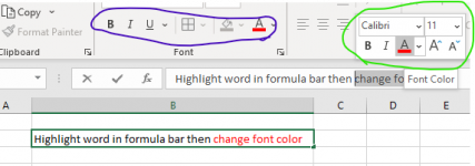
@p45cal You can just select the text in formula bar, then a small box of text formatting(Circled in Green) will appear and you can just change the color or you can use the 1 in ribbon(Circled in Blue)

Font color.png
 
Thanks again everyone!

@ricklinty - I have another question still related to pivot tables. I attached my sample problem to this message. Going forward should I post a brand new thread for each question or is it ok to keep them in the same thread if they are similar?
@accountingguy
I'm not sure should post a brand new thread or keep them in same thread.
For me I will post new thread.
For your second question, normally pivot table won't formatted as below.
Even if can, it needs very complicated transformation and DAX formula
You better do it in your way using formula.
Non normal pivot.png
 
You can just select the text in formula bar, then a small box
I was really after knowing how you got the table with the headers How to Calculate, Pivot Table columns and Formula; is it a table that can be shown by some view or option in Power Pivot? If not, how? Was it a table you typed in yourself? The colour of the text doesn't matter, how did you get the text?
 
I was really after knowing how you got the table with the headers How to Calculate, Pivot Table columns and Formula; is it a table that can be shown by some view or option in Power Pivot? If not, how? Was it a table you typed in yourself? The colour of the text doesn't matter, how did you get the text?
I manually type into a table by copy each Measure's Name and formula
 
Back
Top