leolapa
New member
- Joined
- Jun 3, 2021
- Messages
- 3
- Reaction score
- 0
- Points
- 0
- Excel Version(s)
- 365
The sample schedule below presents 3 sets of bank statements from different accounts/institutions, each one under separate named tables (Stmt1, Stmt2, Stmt3). By using structured referencing it helps the effort of keeping track of the latest balance for each statement as they keep growing over time.
At the very top, cell F1 dynamically sums the latest balance (last populated row) of each statement in order to inform the user the grand total of cash "on hand":
=SUM(LOOKUP(2;1/(Stmt1[Balance]<>"");Stmt1[Balance]);LOOKUP(2;1/(Stmt2[Balance]<>"");Stmt2[Balance]);LOOKUP(2;1/(Stmt3[Balance]<>"");Stmt3[Balance]))
So far, so good........ until there's always a BUT.........
In case I keep opening up new checking/savings/trading accounts and therefore new statements (Stmt4, Stmt5 and so on) start popping up to the right of the existing ones (column O onwards), HOW CAN I MAKE THE FORMULA ON F1 TO AUTOMATICALLY/DYNAMICALLY ADD THOSE NEW NAMED TABLES TO ITS SUM?
The obvious answer on such simple schedule is to just manually copy/paste the LOOKUP formula and change to the newly added table name. However my real life workbook is way more complex than that, and such task would not only be a chore but I also risk forgetting to incorporate those new statements to the tally formula. Thus I need a formula that recognizes as new statements are added so I don't have to worry about doing that in the future, and without recurring to VBA coding or helper columns.
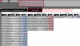
So I started my attempt to get to a solution by naming each table the same + a sequential number 1, 2, 3, etc. as this allows a recognition mechanism as new tables are added. Then I created a SEQUENCE formula based on the COUNTA of statement titles on row 3:
=SEQUENCE(COUNTA($3:$3))
And this enabled me to concatenate the structured referencing for all "Balance" columns on each statement:
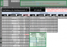
="Stmt"&SEQUENCE(COUNTA(SEQUENCE(SUBTOTAL(3;$3:$3))))&"["&Stmt1[[#Headers];[Balance]]&"]"
And as shown on the screenshot that follows I seemed to be on the right track to get to an INDIRECT "spilled" type solution that should do the trick just fine...
But that's when things started to go south......
I tried 4 different approaches to dynamically pick up the latest balance/last populated row of each statement table, but none of them worked in a way that would provide a dynamic solution that will ensure all future statements be integrated in the sum without further finagling.
My first go was by using the same LOOKUP(2;1/.... approach that returns the last non-empty row of a column. But this one is a no starter as it does not return a cell reference, so SUBTOTAL won't even take it (SUM/AGGREGATE do take nested functions that return values, but won't deal with spilled ranges so they are not feasible options).
=SUBTOTAL(9;LOOKUP(2;1/(INDIRECT("Stmt"&SEQUENCE(COUNTA(SEQUENCE(COUNTA($3:$3))))&"["&Stmt1[[#Headers];[Balance]]&"]")<>"");INDIRECT("Stmt"&SEQUENCE(COUNTA(SEQUENCE(COUNTA($3:$3))))&"["&Stmt1[[#Headers];[Balance]]&"]")))
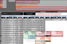
Then I attempted 3 different combinations of INDEX, and they all managed to get to a "spilled" solution but returning ZERO amount, and by decomposing each formula I realized that despite achieving spilled solutions they all return errors.
MAX/ROW:
=SUBTOTAL(9;INDEX(INDIRECT("Stmt"&SEQUENCE(COUNTA(SEQUENCE(SUBTOTAL(3;$3:$3))))&"["&Stmt1[[#Headers];[Balance]]&"]");MAX(ROW(INDIRECT("Stmt"&SEQUENCE(COUNTA(SEQUENCE(SUBTOTAL(3;$3:$3))))&"["&Stmt1[[#Headers];[Balance]]&"]")))-ROW(INDIRECT("Stmt"&SEQUENCE(COUNTA(SEQUENCE(SUBTOTAL(3;$3:$3))))&"[[#Headers];["&Stmt1[[#Headers];[Balance]]&"]]"))))
COUNTA:
=SUBTOTAL(9;INDEX(INDIRECT("Stmt"&SEQUENCE(COUNTA(SEQUENCE(SUBTOTAL(3;$3:$3))))&"["&Stmt1[[#Headers];[Balance]]&"]");SUBTOTAL(3;INDIRECT("Stmt"&SEQUENCE(COUNTA(SEQUENCE(SUBTOTAL(3;$3:$3))))&"["&Stmt1[[#Headers];[Balance]]&"]"))))
INDIRECT/ADDRESS:=SUBTOTAL(9;INDIRECT(ADDRESS(MAX(ROW(INDIRECT("Stmt"&SEQUENCE(COUNTA(SEQUENCE(SUBTOTAL(3;$3:$3))))&"["&Stmt1[[#Headers];[Balance]]&"]")));COLUMN(INDIRECT("Stmt"&SEQUENCE(COUNTA(SEQUENCE(SUBTOTAL(3;$3:$3))))&"["&Stmt1[[#Headers];[Balance]]&"]")))))
It can be seen on each screenshot for every approach that they all do work individually (ORANGE sections), but this way I would get to the same static formula that won't automatically incorporate further statements.
What am I doing wrong here? Is there any other way to go about that I can't seem to grasp? Any help on this is greatly appreciated!
Below I added screenshots for each of the above mentioned INDEX combinations...
INDEX + MAX/ROW:
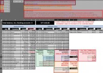
INDEX +COUNTA:
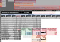
INDEX + INDIRECT/ADDRESS:
At the very top, cell F1 dynamically sums the latest balance (last populated row) of each statement in order to inform the user the grand total of cash "on hand":
=SUM(LOOKUP(2;1/(Stmt1[Balance]<>"");Stmt1[Balance]);LOOKUP(2;1/(Stmt2[Balance]<>"");Stmt2[Balance]);LOOKUP(2;1/(Stmt3[Balance]<>"");Stmt3[Balance]))
So far, so good........ until there's always a BUT.........
In case I keep opening up new checking/savings/trading accounts and therefore new statements (Stmt4, Stmt5 and so on) start popping up to the right of the existing ones (column O onwards), HOW CAN I MAKE THE FORMULA ON F1 TO AUTOMATICALLY/DYNAMICALLY ADD THOSE NEW NAMED TABLES TO ITS SUM?
The obvious answer on such simple schedule is to just manually copy/paste the LOOKUP formula and change to the newly added table name. However my real life workbook is way more complex than that, and such task would not only be a chore but I also risk forgetting to incorporate those new statements to the tally formula. Thus I need a formula that recognizes as new statements are added so I don't have to worry about doing that in the future, and without recurring to VBA coding or helper columns.

So I started my attempt to get to a solution by naming each table the same + a sequential number 1, 2, 3, etc. as this allows a recognition mechanism as new tables are added. Then I created a SEQUENCE formula based on the COUNTA of statement titles on row 3:
=SEQUENCE(COUNTA($3:$3))
And this enabled me to concatenate the structured referencing for all "Balance" columns on each statement:
="Stmt"&SEQUENCE(COUNTA(SEQUENCE(SUBTOTAL(3;$3:$3))))&"["&Stmt1[[#Headers];[Balance]]&"]"
And as shown on the screenshot that follows I seemed to be on the right track to get to an INDIRECT "spilled" type solution that should do the trick just fine...

But that's when things started to go south......
I tried 4 different approaches to dynamically pick up the latest balance/last populated row of each statement table, but none of them worked in a way that would provide a dynamic solution that will ensure all future statements be integrated in the sum without further finagling.
My first go was by using the same LOOKUP(2;1/.... approach that returns the last non-empty row of a column. But this one is a no starter as it does not return a cell reference, so SUBTOTAL won't even take it (SUM/AGGREGATE do take nested functions that return values, but won't deal with spilled ranges so they are not feasible options).
=SUBTOTAL(9;LOOKUP(2;1/(INDIRECT("Stmt"&SEQUENCE(COUNTA(SEQUENCE(COUNTA($3:$3))))&"["&Stmt1[[#Headers];[Balance]]&"]")<>"");INDIRECT("Stmt"&SEQUENCE(COUNTA(SEQUENCE(COUNTA($3:$3))))&"["&Stmt1[[#Headers];[Balance]]&"]")))

Then I attempted 3 different combinations of INDEX, and they all managed to get to a "spilled" solution but returning ZERO amount, and by decomposing each formula I realized that despite achieving spilled solutions they all return errors.
MAX/ROW:
=SUBTOTAL(9;INDEX(INDIRECT("Stmt"&SEQUENCE(COUNTA(SEQUENCE(SUBTOTAL(3;$3:$3))))&"["&Stmt1[[#Headers];[Balance]]&"]");MAX(ROW(INDIRECT("Stmt"&SEQUENCE(COUNTA(SEQUENCE(SUBTOTAL(3;$3:$3))))&"["&Stmt1[[#Headers];[Balance]]&"]")))-ROW(INDIRECT("Stmt"&SEQUENCE(COUNTA(SEQUENCE(SUBTOTAL(3;$3:$3))))&"[[#Headers];["&Stmt1[[#Headers];[Balance]]&"]]"))))
COUNTA:
=SUBTOTAL(9;INDEX(INDIRECT("Stmt"&SEQUENCE(COUNTA(SEQUENCE(SUBTOTAL(3;$3:$3))))&"["&Stmt1[[#Headers];[Balance]]&"]");SUBTOTAL(3;INDIRECT("Stmt"&SEQUENCE(COUNTA(SEQUENCE(SUBTOTAL(3;$3:$3))))&"["&Stmt1[[#Headers];[Balance]]&"]"))))
INDIRECT/ADDRESS:=SUBTOTAL(9;INDIRECT(ADDRESS(MAX(ROW(INDIRECT("Stmt"&SEQUENCE(COUNTA(SEQUENCE(SUBTOTAL(3;$3:$3))))&"["&Stmt1[[#Headers];[Balance]]&"]")));COLUMN(INDIRECT("Stmt"&SEQUENCE(COUNTA(SEQUENCE(SUBTOTAL(3;$3:$3))))&"["&Stmt1[[#Headers];[Balance]]&"]")))))
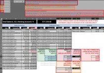
It can be seen on each screenshot for every approach that they all do work individually (ORANGE sections), but this way I would get to the same static formula that won't automatically incorporate further statements.
What am I doing wrong here? Is there any other way to go about that I can't seem to grasp? Any help on this is greatly appreciated!
Below I added screenshots for each of the above mentioned INDEX combinations...
INDEX + MAX/ROW:

INDEX +COUNTA:

INDEX + INDIRECT/ADDRESS:

Last edited:

