Unable to calculate average of a column

Hi everyone,

Good afternoon, Please go through the attachment. what i have and what I want to achieve is as follows
1) There are number of sheets in a excel sheet
2) In one sheet there is a column which has this formula
=IF((VALUE(H6)>0.75),"3",IF((VALUE(H6)>0.5),"2",IF((VALUE(H6)>0.25),"1",IF((VALUE(H6)>0),"0.5","-"))))
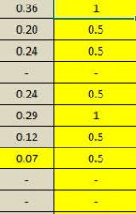
Now after using this formula....the values comes up as 2 or 3 or 1 or 0.5 [this column title is "attainment level"]
3) Now I want to calculate the average of this column at the end cell

What is the problem I am facing?
1) when I give the formula =AVERAGE(I6:I51)....I am getting DIV/0 error
2) Suppose if I copy on this column to other blank sheet and paste as "values only"....still the same problem.
3) In the other sheet the formula is not shown up but there is a green mark indicating "it is not just the value"

Kindly help me to resolve this issue.
In short....how to fetch the formulated columns value only for other formula? "value(H6)" is not working in my case.

Excel sheet is attached. In this excel sheet, I need RED colored column average at its last cell.

Thanks for the help

Values between double quotes are seen by XL as text
In your formula =IF((VALUE(H6)>0.75),"3",IF((VALUE(H6)>0.5),"2",IF((VALUE(H6)>0.25),"1",IF((VALUE(H6)>0),"0.5","-")))) remove double quotes around the numbers (3 instead of "3", etc...) and see if it works
It's always dangerous to manually align cells. Text is always left aligned and numbers are right aligned.
If you align them manually you cannot see the difference anymore

Pecoflyer said:

Values between double quotes are seen by XL as text
In your formula =IF((VALUE(H6)>0.75),"3",IF((VALUE(H6)>0.5),"2",IF((VALUE(H6)>0.25),"1",IF((VALUE(H6)>0),"0.5","-")))) remove double quotes around the numbers (3 instead of "3", etc...) and see if it works
It's always dangerous to manually align cells. Text is always left aligned and numbers are right aligned.
If you align them manually you cannot see the difference anymore

Click to expand...

Thank you Pecoflyer ,
But if I remove the double quotes around the number("3")....then I am getting "#VALUE!" in the place where there are "-". Kindly verify and suggest. Thanks

Hi
pleaqe don't quote entire posts unnecessarily, they make threads hard to read.

But if I remove the double quotes around the number("3")....then I am getting "#VALUE!" in the place where there are "-". Kindly verify and suggest. Thanks

Click to expand...

And which place is that? In col I you can only get a dash if your values in col H are negative
Also keep in mind that when the value in col H is a - the value in I is 3. Is that what you want?

Hi there,
Thanks for the reply.
Let me put the problem in a little bit different way.
Could you please help me to write the formula in the following case?
There are two columns H and I with following data
column H column I
0.72
0.20
0.52
-
You need to write the formula for column I based on following condition
1) If H is > 0.75 then I value should be 3 ( 3 need to appear in I)
2) If H is > 0.5 then I value should be 2
3) If H is > 0.25 then I value should be 1
4) If H is between 0 and 0.25 then I value should be 0.5
5) If H has "-" then I should also need to have "-"
Please see the result expected.

I tried myself, but I know the query is not complete:
=IF((VALUE(H5)>0.75),3,IF((VALUE(H5)>0.5),2,IF((VALUE(H5)>0.25),1,IF((VALUE(H5)>0),"0.5","-"))))
COULD YOU PLEASE CORRECT ME?
Thanks

I used the following in col I =IF(H5="-","-",IF(H5>0.25,FLOOR(H5,0.25)/0.25,0.5))
See attached

View attachment toforum.xlsx

Super Pecoflyer
Thanks a lot. Your solution works.
I will get back if any further help needed.

Once again thank a lot.

You're welcome
If you have any new question, I advise you start a new thread eventually linked to this one. Doing so will increase your chances of a fast answer

Hi Pecoflyer
You have used the formula =IF(H5="-","-",IF(H5>0.25,FLOOR(H5,0.25)/0.25,0.5))

When I paste it to the column I noticed that...for all values it works well (even for "-") but for values less than 0.25, I need to get 0.5 as the answer. This is not happening.
In short if the value in column H is between 0 and 0.25 the corresponding value in I should be 0.5.
Could you please correct it. Thanks
If you have time, kindly explain me the logic which you have used. As per my knowledge the FLOOR is used to round to nearest value. How you used it in my case?
Thanks

Try this instead =IF(H5="-",H5,IF(H5>0.25,FLOOR(H5,0.25)/0.25,0.5))

I'll drop by later for an explanation if you haven't found out yet
Cheers

Thank you very much for your help.

You're welcome