Formula to return multiple matches from multiple columns

Alastair

New member
Joined
Jan 24, 2017
Messages
5
Reaction score
0
Points
0
Location
Sydney
Excel Version(s)
Office 365 Mac
Hi,

I'm hoping someone can assist with a formula that can return multiple matches from multiple columns.

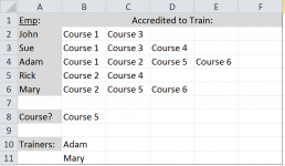
As per the below image (and attached file) A2:A6 contains a list of trainers. B2:F6 contains the various courses that each is accredited to deliver.
What I want to be able to do (as the real file is much larger) is enter the name of a course in B8 and have a list of any trainers accredited to deliver that course appear from B10 downwards. I've manually entered the data in B10:B11 to illustrate what I'm hoping to achieve.

Any assistance would be greatly appreciated.

With thanks,

Al.
Capture.PNG
 

Attachments

  • Book1.xlsx
    12.2 KB · Views: 55
  • Capture.PNG
    Capture.PNG
    8.9 KB · Views: 27
Try this array formula:

=IFERROR(INDEX($A$2:$A$6,SMALL(IF($B$2:$F$6=$B$8,ROW($A$2:$A$6)-ROW($A$2)+1),ROWS($B$10:$B10))),"")

confirmed with CTRL+SHIFT+ENTER not just ENTER, then copied down as far as needed to equal number of trainers.
 
My sincere thanks NBVC.

Your formula works perfectly.

Al.
 
Hi, I'm following NBVC's post as guide but its not working as hoped. I have languages various cells in columns A to L (rows 1-234), countries in column M (rows 1-234), languages in column N (rows 1-222). I want a list of countries matching a each languages in columns from columns O onwards. My formulas for N1, N2 & N3 are:
=IFERROR(INDEX($M$1:$M222,SMALL(IF($A$1:$M$234=N1,ROW($M$1:$M222)-MIN(ROW($M$1:$M222))+1),COLUMNS(O1:O1))),"")

=IFERROR(INDEX($M$1:$M222,SMALL(IF($A$1:$M$234=N2,ROW($M$1:$M222)-MIN(ROW($M$1:$M222))+1),COLUMNS(O2:O2))),"")

=IFERROR(INDEX($M$1:$M222,SMALL(IF($A$1:$M$234=N3,ROW($M$1:$M222)-MIN(ROW($M$1:$M222))+1),COLUMNS(O3:O3))),"")

Formulas for O2 & O3 partly work, they both only give me 1 country, not all. Formula for O1 gives me a blank cell. All languages have at least one language.
How do I get all countries for each language in a row?
 
RichardDunne, you really need to supply a workbook.
 
RichardDunne, you really need to supply a workbook.

screen1.png

screen2.png

I hope workbook attachment are OK. I want to match the languages from column Q with any in the range A1:O235, then select the country from column P on any row that language appears in. I wan to put the the country or countries in a list horizontally starting from column R.
 
I hope workbook attachment are OK.
I can't do anything with a picture of a workbook - I'm not going to start copying the image to a real workbook to start experimenting getting what you want.
A workbook needs to be attached - they end variously in .xls , .xlsx , .xlsb .
 
I'm looking to attach my workbook, according the FAQ Attachments and Images,
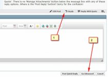
To attach a file to your post, you need to be using the main 'New Post' or 'New Thread' page and not 'Quick Reply'. To use the main 'New Post' page, click the 'Post Reply' button in the relevant thread.
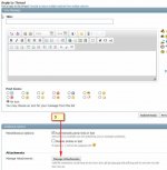
On this page, below the message box, you will find a button labelled 'Manage Attachments'. Clicking this button will open a new window for uploading attachments. You can upload an attachment either from your computer or from another URL by using the appropriate box on this page. Alternatively you can click the Attachment Icon to open this page.
There are only three reply options I see, 'Reply to Thread', 'Quick Reply' and 'Reply With Quote'. There is no 'Manage Attachments' button below the message box with any of these reply options. Where is the 'Post Reply' button? Sorry for the confusion!
 
2017-02-05_014621.JPG
2017-02-05_014740.JPG
2017-02-05_014845.JPG
2017-02-05_014944.JPG
2017-02-05_015126.JPG
 
Last edited:
Thanks for that.
I have attached the excel sheet. Just to clarify, which ever rows the languages in column in column Q appear in from rows A to O, I want o select the country from that row or rows and list them horizontally from column R. Hope that helps.

Richard.
 

Attachments

  • Language.xlsx
    27.5 KB · Views: 41
Your formula was very nearly correct.
The Name CountryList needed to be made absolute.

New formula in R1 needs to be array-entered (Ctrl+Shift+Enter, not just Enter):
Code:
=IFERROR(INDEX(CountryList,SMALL(IF(LanguageRange=$Q1,ROW(LanguageRange)),COLUMN()-17)),"")
then copied across and down.

Many of the cells in your data have leading spaces which would cause the results to be incomplete. I have removed all of them.
You have, on row 213, both English and Tongan listed twice, which causes them to be listed twice in the results. I have not removed these double entries.

Formulae are complicated, and these are all array-formulae, so the sheet is quite resource-hungry (it takes significant time to recalculate the sheet).

On a second sheet which I've added (Pivot) I have re-arranged your data into columns A and B, then used that as a database for a pivot table starting at cell D1.
Now you have many more ways to display your data and it's much less resource-hungry.
 

Attachments

  • ExcelGuru7344Language.xlsx
    321.9 KB · Views: 19
Last edited:
I'm perplexed why the formula didn't return values for all languages as it should. Thanks again. I'll revert back.
 
The pivot table is certainly a different way of doing it! It does the job!
It might be a pointless task but I am looking at an alternative approach as well without the iferror(), as I know each language has an associated country. Cheers.
 
I'm perplexed why the formula didn't return values for all languages as it should. Thanks again. I'll revert back.
The pivot table is certainly a different way of doing it! It does the job!
It might be a pointless task but I am looking at an alternative approach as well without the iferror(), as I know each language has an associated country. Cheers.
Oops, there are some languages in column Q which have leading or trailing spaces which I forgot to check for.
Eg. Assyrian, cell Q11, has a space at the end or beginning; remove it and Iraq pops up in the adjacent cell.
The IfError isn't for the first column (R), it's for all the columns to the right where we don't know whether there'll be countries or not. The formulae have to extend to the right to cover for the max number of countries, which is 100+ for English. The formulae need to be copied further over than the file I included last, up to column DZ. So there are very many cells with formulae returning errors which need to be blank.
 
In the attached, I've extended the formulae further to the right to column EA, removed all leading and trailing spaces (and if there were any double spaces between words they've gone too) over the entire data on Sheet1, removed the double Tonga entries, updated the pivot source data, left a couple of macros in there: one to remove errant spaces from whatever cells are currently selected, the other to re-arrange the data into columns A and B of the Pivot sheet.
The file is an xlsb file to make it small enough to attach (it's big because of all the formulae, not because of the pivot table).
 

Attachments

  • ExcelGuru7344Language.xlsb
    451.9 KB · Views: 22
Back
Top