Introduction
How many times have you built a table of data, and put totals on it. You ship it out the door, and another user comes along and inserts a new row right before the totals row? If you have seen this in play, you'll know that the new row is actually inserted between the end of the data range and the totals row, meaning that your sum formula no longer picks up the entire range of data!
Fortunately, the issue with missing rows in totals can easily be fixed so that a user can insert a row immediately above your totals without missing the last line(s). Here's how:
Create a named range
The first thing we need to do is select a cell on our worksheet other than cell A1. So select cell A2 now, and create the name in your version of Excel as shown below:
Excel 97-2003
- Go to the Insert menu, and choose Name --> Define
- Enter the name CellAbove
- Change the formula to =A1
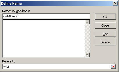
- Click Add
Excel 2007+
- Go to the Formulas tab, and choose Define Name from the Defined Names group
- Enter the name CellAbove
- Change the Scope to the current sheet
- Change the Refers To formula to =A1
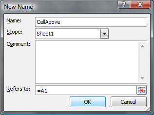
- Click OK
Test the output
If you've followed the steps above correctly, you have now created a named range that can be used as a formula anywhere on the sheet. The key to this was removing the $ signs from the formula, as those would create an absolute cell reference. Without them, we have a relative cell reference that can be used anywhere you are in the worksheet. As you had your cursor in cell A2, and referred to cell A1, the relative reference really points to the cell above the selected cell.
Let's try it out.
- Go to any cell on the sheet, and enter some data.
- In the cell immediately below the one you entered data into, enter =CellAbove and press Enter.
You should now see the same data (numbers, text, or whatever you entered,) in the two cells. Try it again with different cells!
Practical Use
Let's mock up a scenario like our original problem.
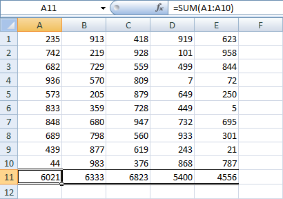
- Create a table from A1:E10 with some random numbers in it;I
- In cells A11, enter the following formula: =Sum(A1:A10)
- Copy the formula in cell A11 to cells B11:E11
We now have a table which, as shown in the formula bar of the image below, has a formula which encompasses all the cells above.
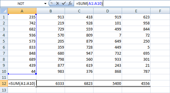
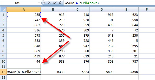
Now, right the row number for row 11 and choose Insert. You will notice that your totals row shifts down, but look in the formula bar now? See how it still only refers to A1:A10? In the picture below, I've clicked inside the formula so that it outlines the area that the formula covers (the blue outline):
Now, let's fix this little problem using our new named range. Change the formula in cell A12 to read =Sum(A1:CellAbove). Notice that now when we click in the formula for this cell it shows us the starting point highlighted in one color, and the ending point of the sum range shown in another colour.
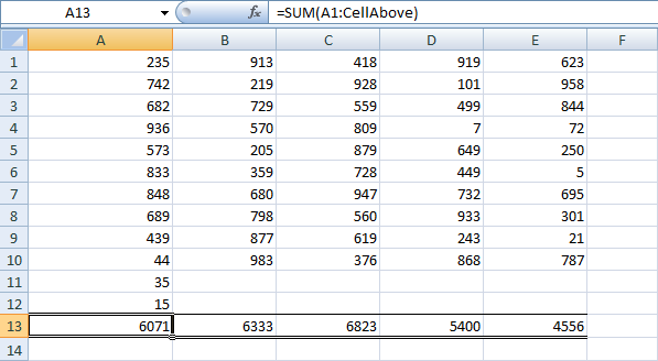
Try entering a number in cell A11 (which is currently blank), and you'll see that it adds into the sum formula.
Now, let's prove that it works... Right click row 12 and choose Insert. The totals row will move down another row. Enter a number in row 11, and voila! It adds into the total!
Caveat
One thing to be aware of is that named ranges created in this way are local to each worksheet. So if you want to use this formula throughout your workbook, you'll need to reproduce the same named range on each worksheet.
As always, if you run into issues with named ranges, and you need to track down a rogue named range, I recommend Jan Karel Peiterse's Name Manager.